Application
Gempy-drivers gives ANALYST users the ability to run GemPy’s geological modeling engine through a ui.json dialogue. The user selects data constraining the model and any options controlling the process. Upon execution, gempy-drivers will reformat the data and make an API call to GemPy, collect the results and re-package into geoh5py objects for display in ANALYST.
Methodology
GemPy’s implicit modeling engine is based on a cokriging method ([LaCM97], [CCCG08]). Geological information in the form of contact, orientation and fault markers are interpolated as a 3D scalar field that represents boundaries between geological domains. See the GemPy Documentation page for more details.
GemPy supports two main types of observations. The first is a contact observation that lies within the surface that it describes. The contact points can either contain orientation data or not. The second type is an orientation observation that may either be within a surface or not.
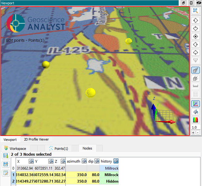
GemPy observation types: A contact point (left), an orientation in a contact (right) and an orientation not in a contact (middle).
There are three types of geological events supported by Gempy: stratigraphy, faults and unconformities. In the absence of faults or unconformities, stratigraphy events are considered conformal and will belong to the same structural group. Faults belong to their own group and are not considered conformal. To model distinct stratigraphic series that are not conformal with each other, a fault or unconformity must separate the stratigraphy events in the reference map representing history.
There are a few rules that need to be followed to generate a valid structural stack in GemPy. The first is that every event must contain at least one contact point. The second is that each conformal group must contain at least one orientation. The gempy-drivers package includes an input validation layer that will catch these user errors and provide a useful error message suggesting how to fix the problem.

Before running gempy-drivers on this data, the user will have to provide at least one orientation, and set at least one point as a contact. If run by mistake, gempy-drivers will fail to run while indicating that it’s missing both a contact point for the Mississippi surface and orientation for the structural group.
Input
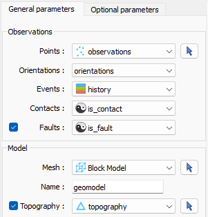
gempy-drivers dialogue.
Observations
The constraining data must be organized into a points object and selected in the dialogue. Creating or adding vertices to a Points object is done with P + left-click in the ANALYST viewport.
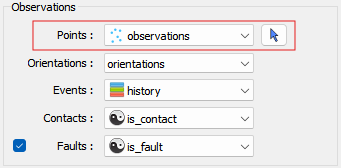
Points object containing constraining data.
The observations object must contain data for orientations, contacts and history, and may optionally also contain data for faults and unconformities.
Constraining data.
These can be created by right-clicking on the points object and opening the script dialogue.
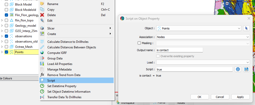
Using scripting to initialize data channels.
Orientations
Orientation data are provided by azimuth and dip channels collected into either a strike and dip or dip direction and dip group. Users can create the azimuth and dip channels from the script menu by providing a float value.
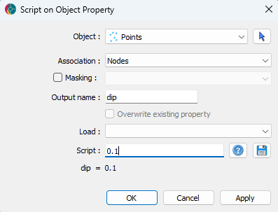
Creating the dip data channel.
Both the azimuth and dip channels can then be collected into a group by right-clicking the observations object, selecting Group Data and choosing one of the special types Strike & dip or Dip direction & dip.
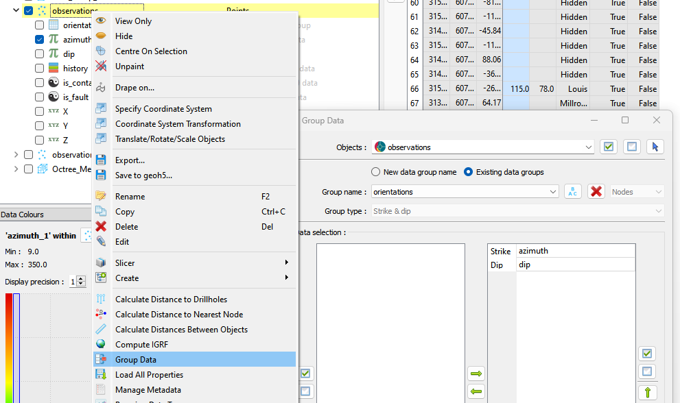
Creating the orientations group.
Contacts, Faults and Unconformities
The contacts, faults and unconformities data channels can be created by providing a true or false value in the script dialogue.
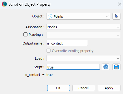
Creating the contacts data channel.
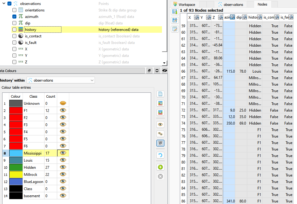
History
The history is represented by a reference data object and is created by providing a string in the script dialogue. The string should contain the name of the event that the point is describing.
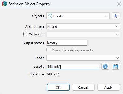
Creating the history data channel.
To add other events categories to the history map, the user can save the references to disk, edit the file to add the new definitions, and then re-load back to the project.

Adding new categories by saving to disk and re-loading. Circled buttons are (top) save and (bottom) load.
The history map must be ordered in geological time so that the oldest event is at the bottom of the list.
Mesh
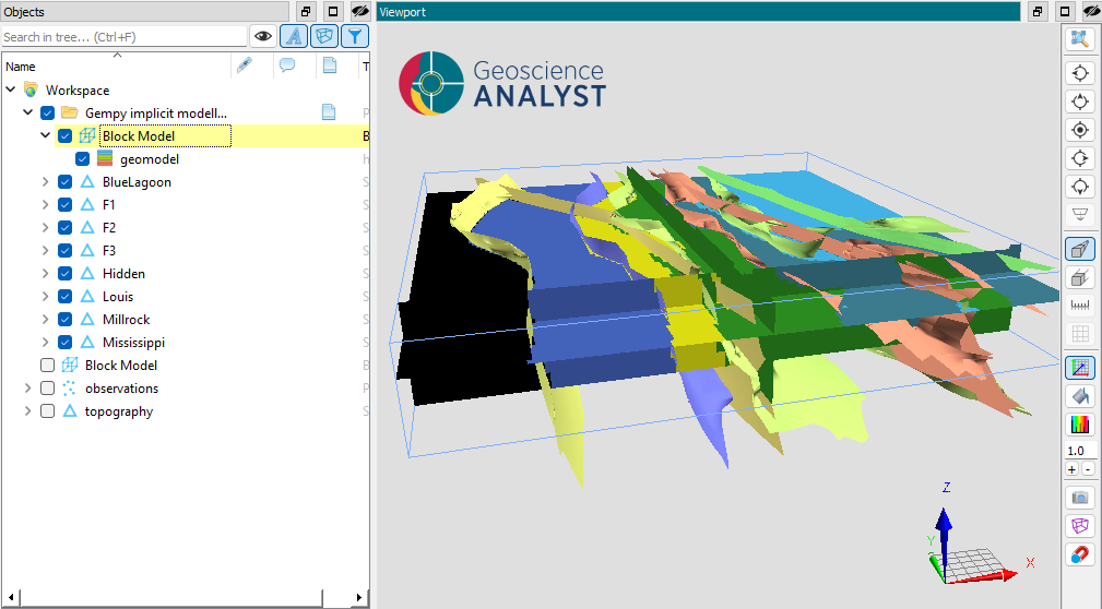
The main artefact of a gempy-drivers run is a geological model defined inside a mesh. The mesh may be optionally provided as a BlockModel or Octree object. If the mesh is not provided, the model is returned inside the Octree mesh internally generated by GemPy. This mesh has the advantage of containing refinement along the implicit modelling surfaces, and is a good choice for initial modelling attempts where efficiency is a priority.
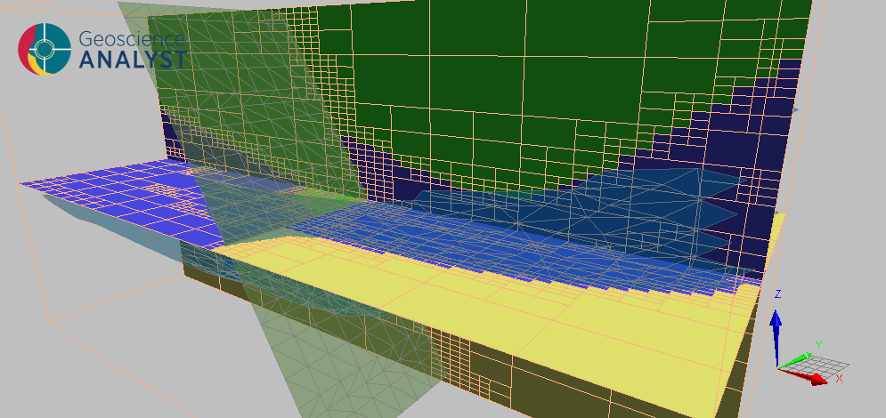
Example of the internal octree mesh created by GemPy.
The trade-off is that the internal meshing does not allow for detailed control over refinement, padding, etc.. Users may only provide the cell sizes in each direction.
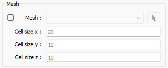
Options for passing pre-constructed meshes or exporting internal GemPy octree meshes.
Model
The geological model is always returned in either the provided mesh or the internal Octree mesh. It may be given a name through the Name field in the dialogue.
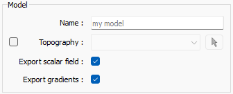
Options for saving lithology and optional scalar field and gradient models.
Topography may be used to clip the top of the model by selecting a surface in the Topography field. Optionally, the scalar field and its gradient may be returned by checking the Export scalar field and Export gradients boxes. For the scalar field options, the mesh will contain a model displaying the scalar field in each cell.
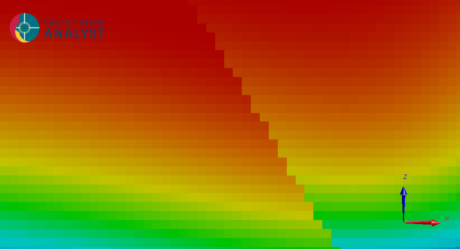
Exported scalar field model.
The scalar field gradient option will add orientation data to both the mesh and observations that shares the property group type of the input data.
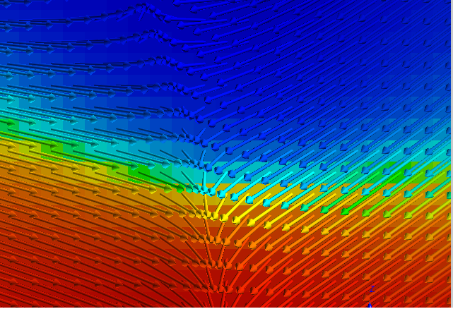
Exported scalar field gradient markers over top of the magnitude.
Additionally, gempy-drivers will also compute the sum-squared residual of the input and output orientations and return a gradient residual channel alongside the output gradient data.
This way users may locate large residuals where the computed orientations don’t match the input and begin to refine their strategy to improve the fit.
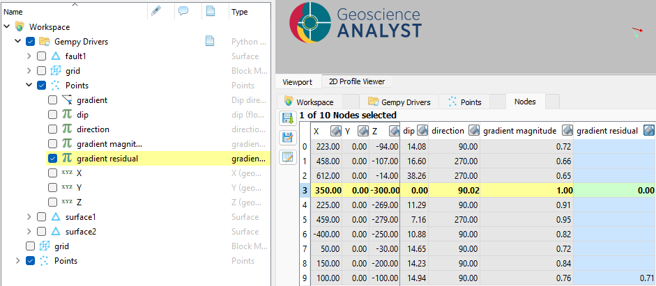
Exported gradient residual computed as the sum squared difference of the input orientations and scalar field gradient.
Interpolation Options
There are a few options available to control the implicit modelling process. These options are in the optional parameters tab of the ui.json interface and are described below.
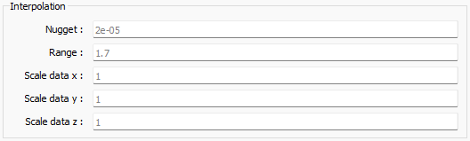
Interpolation options.
Nugget
The nugget effect controls how closely the model fits the contact points. The nugget can be applied globally or heterogeneously across all the observation points. The default value is 1e-5 (globally), which pushes the model to fit contact points closely under normal circumstances. Smaller values will fit contact points more closely and larger values allow the model to deviate more from the contact points to obey orientation data. In the example below we demonstrate the nugget effect for a set of contact points describing horizontal bedding, but with a single outlier point.
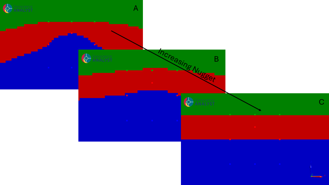
Increasing nugget effect with and outlier contact point and a single horizontal orientation.
The default nugget value is small and forces the model to fit the outlier contact point (A). In some cases, this may not be desired as observations can be noisy and potentially erroneous. By increasing the nugget, the fit to the contact points will be relaxed and result in something like a ‘best fit’ middle layer interface (B). As the nugget increases further, the model will tend towards fitting the orientation data. Since the example uses a single flat orientation data marker, the model will tend towards horizontal bedding (C).
Range
The range parameter controls how much surfaces can bend to fit the observations. The default value is 1.7, which is a good moderate value for many models when accompanied by the default nugget value. In cases where the model cannot fit contact points at a given nugget value, decreasing the range may help improve the fit. In the example below we demonstrate the effect of decreasing the range for the same set of observations as above, but with a large nugget effect such that the default range (A) fails to accurately fit the outlier contact point. Decreasing the range at the same nugget value allows the middle layer interface to bend in order to fit the outlier more closely (B). Further decreasing the range allows the fit to improve, but results in unjustified bending in the corners of the model (C).
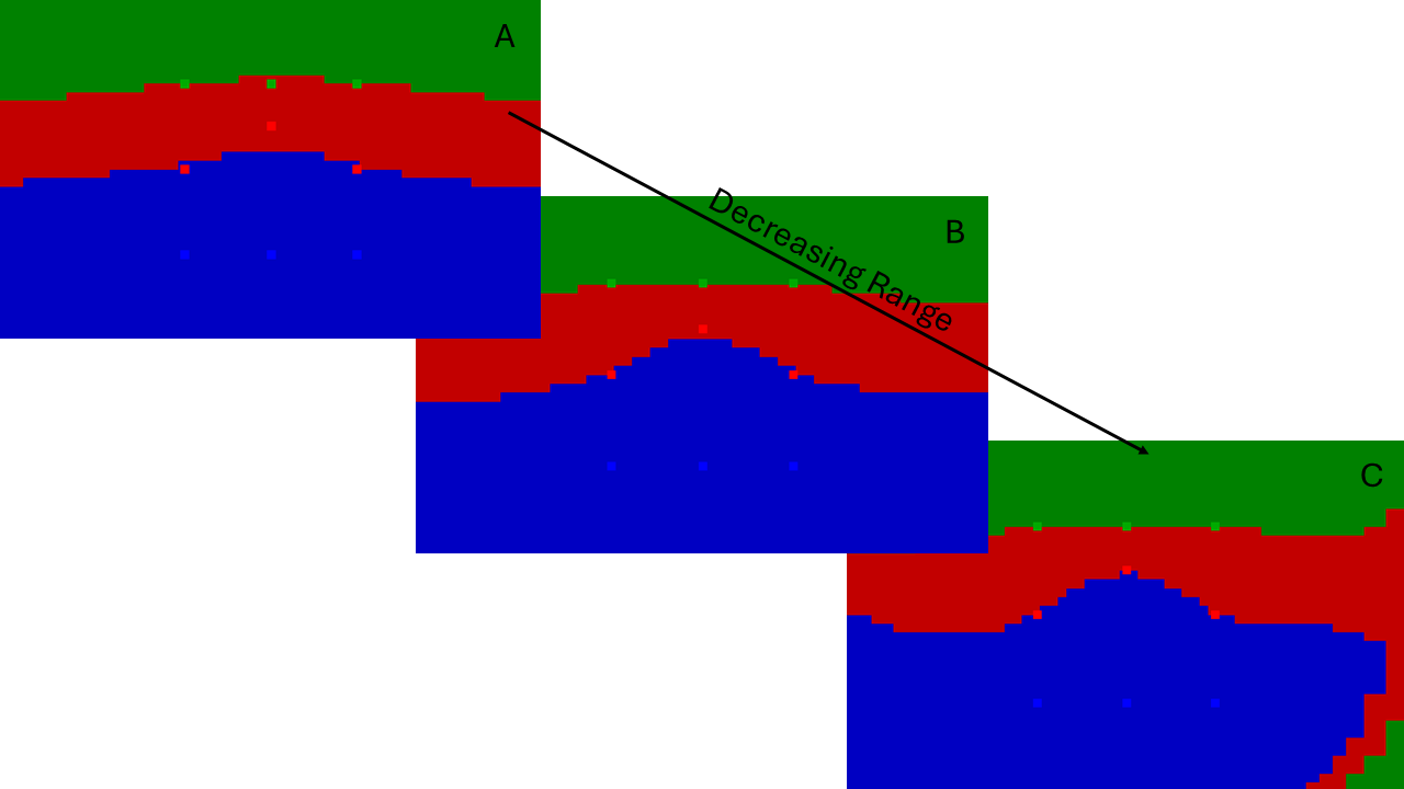
Decreasing the range allows the interfaces in the model to bend more to fit contact points.
Scale data
The scale parameters allow users to re-scale the data independently in each direction. The coordinates of each axis will be multiplied by their provided scale factor. A factor of one keeps the data in its original form, and greater than one stretches the data out in that dimension. GemPy will always transform the data to the unit cube before modelling, so all that matters is the relative spacing in each dimension. GemPy also handles conversion after modelling so the results will always be in the original coordinate system.
The scale parameters can be useful in cases where the observations are anisotropically distributed. For example, if the data are contained in drillholes that are kilometers apart, but the layer markers are only meters apart. In this scenario, scaling the data vertically proportional to the aspect ratio of the drillhole spacing to the layer thickness allows the scalar range parameter to apply in all dimensions equally and can greatly improve results.
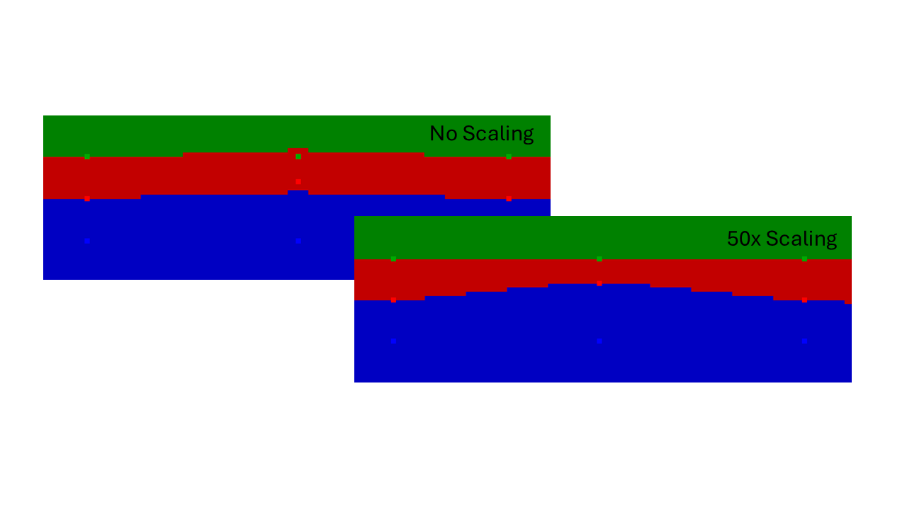
Scaling the z coordinates of the data by 50x to even out the aspect ratio of the observations allows the interpolation to fit the outlier using the default range.
Output
The output of the gempy-drivers is a geological unit model, stored as Referenced data on the input mesh, and a set of surfaces that describes the geological model. The surfaces and model are stored in a UIJson group container.
Output from gempy-drivers.
References
Lajauni, D.; Courrioux, G.; Manuel, L.: Foliation fields and 3D cartography in geology: Principles of a method based on potential interpolation. Math Geol 29, 571-584 (1997).
Calcagno, P.; Chilès, J.P.; Courrioux, G.; Guillen, A.: Geological modelling from field data and geological knowledge: Part I. Modelling method coupling 3D potential-field interpolation and geological rules, Physics of the Earth and Planetary Interiors 171, 147-157 (2008).